Restricted Boltzmann Machine
Restricted Boltzmann Machine (RBM) is a stochastic autoencoder that can serve as feature encoder and/or decoder.
One of its uses is initialization of weights of a neural network prior to its actual training via stochastic gradient descent (SGD), using e.g. back-propagation for (fine) tuning.
When used like this, RBMs are stacked on top of each other to form a deep belief network (DBN).
This is why RBM in Brain Simulator is built upon the classic neural network hidden layer. RBM layer inherits its whole functionality and thus can be used as both autoencoder and as a part of any neural network.
Model
RBM is a two-layer neural network.
The two layers are fully connected to each other, there are no inner connections inside the layers.
The input layer is also called visible layer, the output layer is hidden.
Visible layer is typically bigger than the hidden layer, since the visible layer represents input and reconstructions while the hidden layer neurons correspond to features of the input.

For more details and a nice high-level example, see Introduction to RBMs by Edwin Chen.
More mathematically precise overview and introduction is available in chapter two of Hinton's paper on training RBMs.
Algorithms
Training and filters
Training is done using the k-step Contrastive Divergence algorithm, first proposed by Hinton.
In the Brain Simulator implementation, training is done in the RBM Learning task.
During training, RBM automatically adjusts its weights based on what it perceives. The weights to one output neuron correspond to one feature of the input entity.
Why? Imagine that the input is a 20x20px grayscale image. The input layer has thus 20x20 = 400 neurons.
Now there are also 400 weights leading to that output neuron; each weight originates in one particular input pixel. And each weight has also a value that determines strength of that connection.
Thus, we can draw these weights as an image too – and each pixel will show us how much the input pixel contributes to activation of this output neuron!
This is why we talk about filters and why we can (and should) represent the weights (the filters) as images.

Above is an example of filters learned on the full MNIST dataset. There are 100 hidden neurons and thus hundred visible filters. The red and yellow overlay is an activation mask. The more red, the more activated the neuron is (consequently, black-and-white neurons aren't activated at all or are activated marginally).
Reconstruction
Remember that weights leading to each output neuron correspond to one filter, since it is a mapping from the input (e.g. from an actual image) to one value, the activation of the output neuron.
Thus, when reconstructing, the value of the output neuron means how much the input correponds to the neuron's filter. If the neuron is active, we can say that the input has a certain feature corresponding to this neuron.
Use RBM Reconstruction task of the RBMGroup (see below).
RBM Group
Any Brain Simulator network that uses RBM layers must be created under the RBMGroup node.
The group itself handles proper flow of data inside the network as long as it is in the RBM mode (doing of the two RBM tasks).
The other possibility is to use various types of SGD available in the group, since the group itself is a descendant of the Neural Network group. You can switch between the modes during runtime.
Parameters
One important thing to note is that RBMs are rather volatile and even small changes in parameters can result in huge differences in performance and behaviour.
Parameters on the left are specific to tasks, not to the node itself. Thus, parameters of RBM Learning and RBM Reconstruction (these are the two possible RBM tasks) are completely different instances of the same concept, meaning that changing CurrentLayerIndex in one won't change it in the other task.
Learning parameters
The learning parameters should be self-explanatory. For their more detailed comparison and discussion about optimal settings, see Hinton's paper on this topic.
In our experience, it generally works well to work with a low learning rate (at most 0.01). However, this might not be true in all cases (but it, so far, has been).
Layer indexing
Layers are indexed from 0 (zero) including.
First layer is always of type RBMInputLayer and its index is 0.
All other layers are RBMLayer and their indices can range from 1 to total number of layers excluding.
In Learning mode, the CurrentLayerIndex parameter is the index of the visible layer.
Let's say we have three layers: one input layer and two RBM layers. If we set CurrentLayerIndex to 0, we will learn weights between input layer (layer 0) and first RBM layer (layer 1).
We can set CurrentLayerIndex to 1 and learn weights between the second layer pair.
We can't set the index parameter to any other value.
In Reconstruction mode, we can either start our sampling on the input layer and then the index says to which layer should we continue before returning back.
We can also start sampling on any other layer (by changing Reconstruction source from INPUT to HIDDEN). In that case, we start at layer specified by index parameter and go all the way back to the input layer and then again forward to the specified layer.
Activation parameters
In RBM, each neuron is assigned a probability of being activated. RBM can work with these probabilities or use random activations to either fully activate the neuron (set its output to 1) or to turn it off (0).
Learning in RBM is based on random activations which theoretically results in good generalization of the model. Random activations can be turned on and off during both training and reconstruction.
RandomVisible and RandomHidden properties obviously determine whether the currently visible and hidden layer will be randomly activated.
RandomPrevious enables or disables random activations of all other layers, i.e. those layers who currently aren't visible or hidden. Thus, this settings only takes effect when there are three or more layers present and we are not working with the first two layers.
Additionally, the SigmoidSteepness parameter is the $\lambda$ parameter in the sigmoid function:
$\sigma(x) = \frac{1}{1+ e^{-x * \lambda}}$
Sigmoid function is used to compute the probability of activation of a given neuron after summing its inputs.
Node parameters
The parameters described above are specific to RBM tasks. The RBM group itself has parameters (by default to the right). However, these parameters are derived from the NeuralNetwork group and only take effect when a task unrelated to RBM is active.
Note that this applies to the Dropout group parameter as well. RBM layers do have dropout too, but it's a layer-specific parameter (see below). The group Dropout parameter has no effect during RBM tasks.
RBM layer
RBM layer is built upon the hidden layer from neural network. The RBMInputLayer is the same except it has no weights and number of neurons is automatically determined from its input.
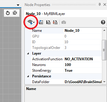
RBM layer features a RBMFilterObserver that enables you to visualize the learned filters. Click here to add it:
Parameters
The only really important parameters are Neurons, which unsurprisingly determines number of neurons in the layer and Dropout, which sets the dropout rate. Note that dropout rate of 0.2 means that 20% of neurons will be dropped out.
ActivationFunction parameter is only used in non-RBM tasks.
Examples
There is an example tutorial as well as a brain file with a two-layer RBM trained on the MNIST dataset.
Additionally, an animated image of visualized filters when learning RBM on MNIST from scratch is available (warning - 100 MB file) here.